Photo by John Fornander on Unsplash

For a game thought of as quintessentially British, with Wimbledon almost arrogantly being known as just ‘The Championships’, I was surprised to know that it probably has its roots in medieval 12th century France (although Brits aren’t really strangers to stealing stuff from other cultures). It appears that the origins of ‘love’, ‘15’, ‘30’ and then the bizarre jump to ‘40’ are a bit mysterious, but all in all the origins are roughly traced with this great article from Time condensing down a lot of the information.

What is interesting (and I can’t seem to find much info on) is how it was settled that a game (not a match) of tennis, would essentially be a race to 4 points — if we forget about ‘deuce’ for now. Regardless of what we call the points, that is essentially what a game is: first to 4. And with this brings the question — what would tennis look like if it was a race to some other number of points? Like 6? Or 8? Or what about just 1 game with a race to 100?

It turns out that choosing 4 points works out very nicely and to show this we can revert to the old ‘Problem of Points’.

What is the Problem of Points?

A classical probability problem that arguably led to the concept of ‘Expected Value’, the Problem of Points (PoP from here on out) concerns the following issue:

“Given a race to _n_ points between 2 players, _a_ and _b_, if player _a_ has _x_ points and player _b_ has _y_ points and we are forced to stop the game right now - how should we split up the prize between the 2 players?”

To take an easy example for illustration — if we have two players that are equally likely to win any given point and they also have the same number of points currently, then we should split the pot 50/50 i.e. each one has a 50% chance of winning. Things become tricker when we start considering:

• unequal probabilities of winning a given point e.g. player a has a 70% chance of winning vs player b’s 30% chance
• unequal current points e.g. player a has 10 more points currently than player b

This is the problem that Pascal and Fermat first discussed.

The solution lies in how many points each player still needs

The key is not how many points each player currently has, x and y, but how many each player needs to win the game i.e. (n-x) and (n-y). This is intuitively clear if we take two games where the score is:

• 8–4, first to 10
• 18–14, first to 20

Clearly the first player has the same chance of winning in each vs the second player.

Solving with equal chance of winning a given point

If we annotate instead the remaining points each player needs as x and y (instead of points won), then we can get the following conclusion: if we play x + y - 1 more points then 1 player must have won. As an example, if a needs x=2 and b needs y=4 then after 5 points either:

• a will have won at least 2 and the game will be over
• b will have won at least 4 and the game will be over

In fact, for an outcome with equal probability we can express the ratio of chances of a:b as:

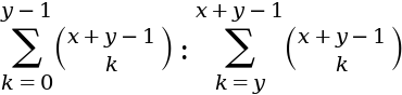
Image by author

In words we can express the above as the following: each side sums up all the possible combinations where either player a (left) or player b (right) wins if we play x+y-1 points i.e. enough points that one player must win. Let’s take a concrete example to demonstrate. Let’s take:

• x=2: player a needs 2 points to win
• y=4: player b needs 4 points to win

Looking at the left hand side we have:

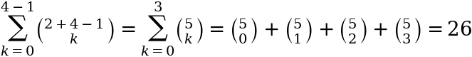
Image by author

In words we count all the times where player b does not win enough points to win i.e. they need 4 to win so we count all the times where they win less than 4 and by definition on these times player a must win. Similarly looking at the right hand side we get:

Image by author

where this time we are counting the number of times where player b does win enough points to win. To convert these counts into probabilities we then need to divide by the total number of occurrences - i.e. the sum of the left and right sides. Fortunately we can make use of Pascal’s Identity which states (in this context):

Image by author

where:

• the first equality comes from combining the summations
• the second equality comes from the sum of the binomial coefficients formula — good proof of this by induction here

Returning to our numeric example above we get probabilities of 26/(2⁵) and 6/(2⁵).

What about when we have unequal probabilities?

Previously we had equal probability of a and b winning any given point - this is like an ‘unweighted’ example that meant to convert to probabilities we just had to divide by the total number of combinations - without weighting the probability that each combination would occur because the weights would all be equal.

Now we have a ‘weighted’ case. It’s like tossing a coin twice with a winning on double heads and b winning on double tails. If we use a loaded coin that comes back 90% of the time as heads obviously the probability of a winning is much higher than that of b winning, despite the fact there is still only one outcome each that leads to victory (double heads or tails can still only occur once in 2 tosses). The probabilities change but the outcome counts remain unchanged.

To make the amendment we move from binomial coefficients to binomial theorem to get:

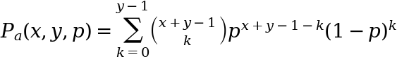
Image by author

where p is the probability that a wins any given point (and correspondingly 1-p for player b) and so P_a is the probability that a wins overall. In words what we are doing here is taking each occasion where player b wins insufficient points (and so player a wins) and:

• counting the number of ways that can happen e.g. there are 5 ways that b can win only 1 point if we play 5 points (they win just the first, they win just the second etc)
• weighting this by the probability that it happens

then finally summing all these together to get the total probability that b wins insufficient points - or in other words that a wins. Given that we are just looking at player a we can also re-write this as:

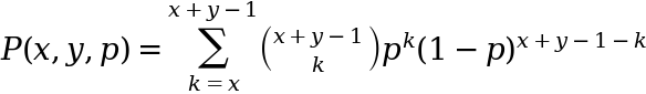
Image by author

This is potentially a more intuitive writing as it expresses the probability that a wins as summing the (probability weighted) occasions when a wins sufficient points.

Riiiight so what does this have to do with tennis?

As mentioned above every game of tennis (again, ignoring deuce) is essentially a race to 4 points. Using the above framework and making the following parallels:

• x: points required for a to win the game with a serving
• y: points required for b to win the game with b returning
• p: probability that a wins a point on their serve

we can then model a game of tennis and play around with x and y to see what happens if we don’t choose a game to be a race to 4 but a race to something else instead.

Given a probability, p, what is the probability that ‘a’ wins a game?

Let’s now use a bit of python to display how the probability of winning a deuce-less game varies as we vary the number of points required to win the game.

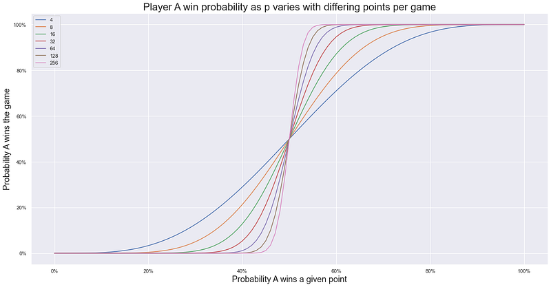
Image by author

So what does the above show? Taking the blue line, this shows how for a ‘first-to-4’ tennis game (closest to standard), how the probability of a winning the whole game varies (y-axis) as we vary the probability that a wins a given point (x-axis). We can see that the effect of upping your probability of winning any given point increases your chance of winning the game by more than 1-for-1 in the middle of the range - just take a look at the fact that:

• 50% chance of winning any point gives 50% chance of winning the game
• 60% chance of winning any point gives >60% chance of winning the game (closer to 70% where the blue line crosses the 60% x-axis)

We can also see that the more points per game, the more sensitive the chance of winning the whole game is to the chance of winning any individual point — shown by the lines getting increasingly steeper around the 50% mark as we add more and more points to the game. In effect we are reducing the randomness of each game as we add more and more ‘trials’ (points) and so increasing the chance that the ‘better player’ (i.e. p>0.5) will indeed prevail. This is similar to The Law of Large Numbers stating that as we add trials the sample mean will approach the population mean. Instead here, as we add trials the probability of the better player winning the game approaches 1 - where we can think of 1 here as the output of an indicator function where:

• 1 means a is the better player
• 0 means b is the better player

What’s the point?

The point is if it was decided that a game of tennis should be a first to 8 race, or more, then we would have a much more boring sport. Every game of tennis has a server and returner and so by definition the server has the advantage. This advantage in professional men’s tennis is around p=65%. If we had longer games then we would have:

• many fewer break points
• as a result much less interesting tennis matches

In fact we can use what we have done above to show this. With p=65% and a tennis game of ‘first-to-4’ we have the probability of being broken as 20%. If we then up the game length to 8 points we end up with this probability dropping to 11.4% - almost half as many breaks. It’s not just the fact that the tennis scoring system is discretised that makes it exciting, it’s that it is discretised into a suitable size of increment that gives the game enough randomness to prevent the slightly better player always winning every time. Which if you are that better player feels unjust, but if you’re anyone else just feels a bit more exciting.